Python for Bioinformatics: A 30-Day Roadmap with 10 Runnable Examples

By Dr. Tamanna Anwar, PhD, Founder, Centre of Bioinformatics Research and Technology (CBIRT)
Python for bioinformatics is easier to learn than most students expect, as long as you learn it in the right order. You do not need a computer science degree. You need about an hour a day, a plan that moves from basics to real biological files, and code you can run yourself from the first day.
This guide gives you both: a 30-day roadmap and 10 short, runnable Biopython examples that cover the tasks you will actually meet in a lab or a job, from translating a gene to filtering sequencing reads and summarizing BLAST results. Every example was tested with Biopython 1.88.
Before you start: set up Python
Install Python 3 and three libraries: Biopython for biological files and sequences, pandas for tables, and matplotlib for plots.
pip install biopython pandas matplotlib
If you use Conda, run conda install -c conda-forge biopython pandas matplotlib instead. Write your code in a plain .py file or a Jupyter notebook. Both work for everything below. Once these feel familiar, our list of the top 30 Python libraries used in bioinformatics shows what to add next.
Still deciding between R and Python? Read our comparison of R vs Python for bioinformatics first. If the field itself is new to you, start with bioinformatics basics.
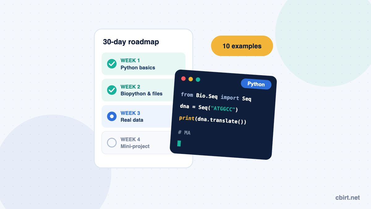
The 30-day roadmap
| Days | Focus | What you should be able to do by the end |
|---|---|---|
| 1–7 | Core Python: variables, strings, lists, dictionaries, loops, if statements, functions, reading and writing text files | Count bases in a DNA string and write the result to a file |
| 8–14 | Biopython basics: Seq, SeqRecord, reading FASTA and GenBank files with SeqIO | Examples 1–5 below, on your own sequences |
| 15–21 | Real data: FASTQ quality, pairwise alignment, downloading from NCBI, tables with pandas, plots with matplotlib | Examples 6–10 below |
| 22–30 | A mini-project from start to finish, published on GitHub with a README | One finished project you can show an interviewer |
Spend the first week on plain Python, even if it feels slow. Most beginners who struggle with Biopython are really struggling with loops and lists.
10 Python examples every bioinformatics beginner should run
For examples 2 and 9, save this as genes.fasta in the same folder as your script:
>geneA sample gene
ATGCGCGATATCGCGCTAA
>geneB
ATATATATGCGCATAT
1. Complement, transcribe and translate a DNA sequence
from Bio.Seq import Seq

dna = Seq("ATGGCCATTGTAATGGGCCGCTGA")
print("Complement:        ", dna.complement())
print("Reverse complement:", dna.reverse_complement())
print("mRNA:              ", dna.transcribe())
print("Protein:           ", dna.translate())
Output:
Complement:         TACCGGTAACATTACCCGGCGACT
Reverse complement: TCAGCGGCCCATTACAATGGCCAT
mRNA:               AUGGCCAUUGUAAUGGGCCGCUGA
Protein:            MAIVMGR*
The * marks the stop codon. This one object, Seq, is the foundation of almost everything else in Biopython.
2. Read a FASTA file and report length and GC content
from Bio import SeqIO
from Bio.SeqUtils import gc_fraction

for record in SeqIO.parse("genes.fasta", "fasta"):
    gc = gc_fraction(record.seq) * 100
    print(record.id, len(record.seq), f"{gc:.1f}% GC")
Output:
geneA 19 52.6% GC
geneB 16 25.0% GC
SeqIO.parse reads one record at a time, so the same three lines work on a file with ten sequences or ten million.
3. Count codon usage
from collections import Counter
from Bio.Seq import Seq

seq = Seq("ATGGCCATTGTAATGGGCCGCTGA")
codons = [str(seq[i:i + 3]) for i in range(0, len(seq) - 2, 3)]
for codon, count in Counter(codons).most_common(3):
    print(codon, count)
Output:
ATG 2
GCC 1
ATT 1
Counter from Python’s standard library is one of the most useful tools in bioinformatics: use it for codons, k-mers, amino acids or gene names.
4. Find open reading frames in all six frames
from Bio.Seq import Seq

seq = Seq("CCATGAAACGCATTAGCACCACCATTACCACCTGAGG")
min_aa = 5  # report open reading frames of at least 5 amino acids

for strand, nuc in [("+", seq), ("-", seq.reverse_complement())]:
    for frame in range(3):
        trimmed = nuc[frame:]
        trimmed = trimmed[: len(trimmed) - len(trimmed) % 3]  # whole codons only
        protein = str(trimmed.translate())
        for piece in protein.split("*"):
            start = piece.find("M")
            if start != -1 and len(piece) - start >= min_aa:
                print(strand, frame, piece[start:])
Output:
+ 2 MKRISTTITT
- 0 MVVLMRFM
The script translates the sequence in three frames on each strand, splits the protein at stop codons, and keeps stretches that start with methionine. It is a simple teaching version; tools such as NCBI ORFfinder handle edge cases for real annotation.
5. Extract genes from a GenBank file
Download any GenBank record from NCBI (choose Send to → File → GenBank on a nucleotide page) and save it as sample.gb.
from Bio import SeqIO

record = SeqIO.read("sample.gb", "genbank")
print(record.id, record.description, len(record.seq), "bp")

for feature in record.features:
    if feature.type == "CDS":
        gene = feature.qualifiers.get("gene", ["?"])[0]
        product = feature.qualifiers.get("product", ["?"])[0]
        protein = feature.extract(record.seq).translate(to_stop=True)
        print(gene, feature.location, product, protein)
For each coding sequence (CDS), this prints the gene name, its location, the product and the translated protein. GenBank files carry annotation that FASTA files do not, and feature.extract handles strands and coordinates for you.
6. Filter sequencing reads by quality
Save any FASTQ file as reads.fastq.
from Bio import SeqIO

def mean_quality(record):
    scores = record.letter_annotations["phred_quality"]
    return sum(scores) / len(scores)

good = (r for r in SeqIO.parse("reads.fastq", "fastq") if mean_quality(r) >= 30)
kept = SeqIO.write(good, "reads.filtered.fastq", "fastq")
print("Reads kept:", kept)
Every base in a FASTQ file has a Phred quality score; a score of 30 means a 1 in 1,000 chance that the base is wrong. This script keeps reads whose average score is at least 30. Real pipelines use dedicated tools such as fastp, covered in our NGS data analysis for beginners guide, but writing it yourself shows you what those tools do.
7. Align two sequences
from Bio import Align

aligner = Align.PairwiseAligner()
aligner.mode = "global"
aligner.match_score = 1
aligner.mismatch_score = -1
aligner.open_gap_score = -2
aligner.extend_gap_score = -0.5

alignments = aligner.align("GATTACAGATTACA", "GATCACAGTTACA")
best = alignments[0]
print("Score:", best.score)
print(best)
Output:
Score: 9.0
target            0 GATTACAGATTACA 14
                  0 |||.||||-||||| 14
query             0 GATCACAG-TTACA 13
| is a match, . a mismatch and - a gap. Change the scores and the mode ("local" instead of "global") to see how the alignment changes. PairwiseAligner replaces the older pairwise2 module.
8. Download a sequence from NCBI
This example needs an internet connection.
from Bio import Entrez, SeqIO

Entrez.email = "you@example.com"  # NCBI asks for your real email address

handle = Entrez.efetch(db="nucleotide", id="NC_045512.2", rettype="fasta", retmode="text")
record = SeqIO.read(handle, "fasta")
handle.close()

print(record.id, len(record.seq), "bp")
SeqIO.write(record, "sars-cov-2.fasta", "fasta")
It downloads the SARS-CoV-2 reference genome (NC_045512.2, 29,903 bp) and saves it as a FASTA file. NCBI asks for an email address so it can contact you if your script causes problems; use your real one.
9. Turn sequence statistics into a table and a plot
import pandas as pd
import matplotlib.pyplot as plt
from Bio import SeqIO
from Bio.SeqUtils import gc_fraction

rows = [
    {"id": r.id, "length": len(r.seq), "gc_percent": gc_fraction(r.seq) * 100}
    for r in SeqIO.parse("genes.fasta", "fasta")
]
df = pd.DataFrame(rows)
print(df.describe().round(2))

df.plot.bar(x="id", y="gc_percent", legend=False)
plt.ylabel("GC content (%)")
plt.tight_layout()
plt.savefig("gc_content.png", dpi=150)
This builds a pandas table with one row per sequence, prints summary statistics, and saves a bar chart of GC content as gc_content.png. pandas and matplotlib are how most bioinformatics results end up in reports and papers.
10. Summarize BLAST results
Run BLAST with tabular output (-outfmt 6) and save the result as blast.tsv. Its 12 standard columns are listed in the code.
import pandas as pd

cols = ["query", "subject", "pident", "length", "mismatch", "gapopen",
        "qstart", "qend", "sstart", "send", "evalue", "bitscore"]
hits = pd.read_csv("blast.tsv", sep="\t", names=cols)

strong = hits[(hits["evalue"] < 1e-10) & (hits["pident"] >= 90)]
best = strong.sort_values("bitscore", ascending=False).drop_duplicates("query")
print(best[["query", "subject", "pident", "evalue"]])
The script keeps hits with an E-value below 1e-10 and at least 90% identity, then reports the best hit for each query. Filtering BLAST output is a daily task in genomics and annotation work.
Common mistakes beginners make
- Skipping plain Python. Biopython makes sense only once loops, lists and dictionaries feel natural.
- Copying code without running it. Type each example, run it, then change one thing and predict the result.
- Reading whole files into memory. Use
SeqIO.parse(one record at a time), not lists of every record, when files get large. - Ignoring warnings. Biopython warns you about partial codons or unusual characters. Read the message; it usually points to a real problem in your data.
- No version control. Put your scripts on GitHub from week one. It becomes your portfolio.
What to build in week four
Pick one project that uses real public data and finish it properly: a README, the data source with its accession number, code that runs from start to finish, and labeled plots. Our list of 10 bioinformatics projects with free datasets has ideas at every level; the FASTA toolkit (project 1) is a natural first step after this roadmap.
Python skills appear in most bioinformatics job descriptions. See our guide to bioinformatics jobs for freshers for the roles they lead to.
Learn Python for bioinformatics with CBIRT
CBIRT’s Python & Biopython for Bioinformatics program is an industry-focused skill development program, taught live online by experienced trainers. You write code on real biological data from the first session, ask questions as you get stuck, finish with an assignment or project, and receive a certificate on completion.
See the Python & Biopython program: dates, fees and registration →
Frequently asked questions
Is Python good for bioinformatics?
Yes. Python is widely used for writing pipelines, processing sequence files, automating analyses and machine learning, and Biopython adds ready-made tools for biological formats such as FASTA, FASTQ and GenBank.
How long does it take to learn Python for bioinformatics?
With about an hour a day, most beginners can write useful scripts within a month, as in the roadmap above. Becoming confident with real projects takes a few more months of regular practice.
Do I need to know programming before learning bioinformatics?
No. Many bioinformaticians start from biology. Learn core Python first, then apply it to biological files straight away.
What is Biopython?
Biopython is a free, open-source Python library for computational biology. It reads and writes biological file formats, handles sequences, runs alignments, and connects to databases such as NCBI.
Should I learn R or Python first?
It depends on your goal. Python suits pipelines, automation and machine learning; R suits statistics and Bioconductor packages. Our R vs Python guide helps you choose.
Sources
- Biopython Tutorial and Cookbook (official Biopython documentation)
- Biopython: Pairwise sequence alignment
- Biopython: Bio.Entrez documentation
- NCBI: BLAST+ command line user manual (tabular output columns)
Related reading on CBIRT: R vs Python for bioinformatics · NGS data analysis for beginners · 10 bioinformatics projects · Bioinformatics course in India